Mamba: The Easy Way
Oxford, UK — February 23, 2024
Shared on Hacker News and X
Today, basically any language model you can name is a Transformer model. OpenAI’s ChatGPT, Google’s Gemini, and GitHub’s Copilot are all powered by Transformers, to name a few. However, Transformers suffer from a fundamental flaw: they are powered by Attention, which scales quadratically with sequence length. Simply put, for quick exchanges (asking ChatGPT to tell a joke), this is fine. But for queries that require lots of words (asking ChatGPT to summarize a 100-page document), Transformers can become prohibitively slow.1
Many models have attempted to solve this problem, but few have done as well as Mamba. Published two months ago by Albert Gu and Tri Dao, Mamba appears to outperform similarly-sized Transformers while scaling linearly with sequence length. If you’re looking for an in-depth technical explanation of Mamba, paired with a full Triton implementation, you’re in the wrong place. Mamba: The Hard Way has already been written by the legend himself, Sasha Rush. If you haven’t heard of Mamba (or Triton), or you’re looking for a higher-level overview of Mamba’s big ideas, I have just the post for you.
The prospect of an accurate linear-time language model has gotten many excited about the future of language model architectures (especially Sasha, who has money on the line). In this blogpost, I’ll try to explain how Mamba works in a way that should be fairly straightforward, especially if you’ve studied a little computer science before. Let’s get started!
Quadratic attention has been indispensable for information-dense modalities such as language... until now.
— Albert Gu (@_albertgu) December 4, 2023
Announcing Mamba: a new SSM arch. that has linear-time scaling, ultra long context, and most importantly--outperforms Transformers everywhere we've tried.
With @tri_dao 1/ pic.twitter.com/vXumZqJsdb
Background: S4
Mamba’s architecture is based primarily on S4, a recent state space model (SSM) architecture. I’ll summarize the important parts here, but if you want to understand S4 in more detail, I would highly recommend reading another one of Sasha’s blogposts, The Annotated S4.
At a high level, S4 learns how to map an input \(x(t)\) to an output \(y(t)\) through an intermediate state \(h(t)\). Here, \(x\), \(y\), and \(h\) are functions of \(t\) because SSMs are designed to work well with continuous data such as audio, sensor data, and images. S4 relates these to each other with three continuous parameter matrices \(\mathbf{A}\), \(\mathbf{B}\), and \(\mathbf{C}\). These are all tied together through the following two equations (1a and 1b in Mamba’s paper):
\[\begin{align}h'(t)&=\mathbf{A}h(t)+\mathbf{B}x(t)\\y(t)&=\mathbf{C}h(t)\end{align}\]
In practice, we always deal with discrete data, such as text. This requires us to discretize the SSM, transforming our continuous parameters \(\mathbf{A}\), \(\mathbf{B}\), \(\mathbf{C}\) into discrete parameters \(\mathbf{\bar{A}}\), \(\mathbf{\bar{B}}\), \(\mathbf{C}\) by using a special fourth parameter \(\Delta\). I’m not going to get into the details of how discretization works here, but the authors of S4 have written a nice blogpost about it if you’re curious. Once discretized, we can instead represent the SSM through these two equations (2a and 2b):
\[\begin{align}h_t&=\mathbf{\bar{A}}h_{t-1}+\mathbf{\bar{B}}x_t\\y_t&=\mathbf{C}h_t\end{align}\]
These equations form a recurrence, similar to what you would see in a recurrent neural network (RNN). At each step \(t\), we combine the hidden state from the previous timestep \(h_{t-1}\) with the current input \(x_t\) to create the new hidden state \(h_t\). Below, you can see how this would work when predicting the next word in a sentence (in this case, we predict that “and” follows “My name is Jack”).

In this way, we can essentially use S4 as an RNN to generate one token at a time. However, what makes S4 really cool is that you can actually also use it as a convolutional neural network (CNN). In the above example, let’s see what happens when we expand the discrete equations from earlier to try to calculate \(h_3\). For simplicity, let’s assume \(x_{-1}=0\).
\[\begin{align}h_0&=\mathbf{\bar{B}}x_0\\h_1&=\mathbf{\bar{A}}(\mathbf{\bar{B}}x_0)+\mathbf{\bar{B}}x_1\\h_2&=\mathbf{\bar{A}}(\mathbf{\bar{A}}(\mathbf{\bar{B}}x_0)+\mathbf{\bar{B}}x_1)+\mathbf{\bar{B}}x_2\\h_3&=\mathbf{\bar{A}}(\mathbf{\bar{A}}(\mathbf{\bar{A}}(\mathbf{\bar{B}}x_0)+\mathbf{\bar{B}}x_1)+\mathbf{\bar{B}}x_2)+\mathbf{\bar{B}}x_3\end{align}\]
With \(h_3\) calculated, we can substitute this into the equation for \(y_3\) to predict the next word.
\[\begin{align}y_3&=\mathbf{C}(\mathbf{\bar{A}}(\mathbf{\bar{A}}(\mathbf{\bar{A}}(\mathbf{\bar{B}}x_0)+\mathbf{\bar{B}}x_1)+\mathbf{\bar{B}}x_2)+\mathbf{\bar{B}}x_3)\\y_3&=\mathbf{C\bar{A}\bar{A}\bar{A}\bar{B}}x_0+\mathbf{C\bar{A}\bar{A}\bar{B}}x_1+\mathbf{C\bar{A}\bar{B}}x_2+\mathbf{C\bar{B}}x_3\end{align}\]
Now, notice that \(y_3\) can actually be computed as a dot product, where the right-hand vector is just our input \(x\):
\[y_3=\begin{pmatrix} \mathbf{C\bar{A}\bar{A}\bar{A}\bar{B}} & \mathbf{C\bar{A}\bar{A}\bar{B}} & \mathbf{C\bar{A}\bar{B}} & \mathbf{C\bar{B}} \end{pmatrix}\begin{pmatrix} x_0\\ x_1\\ x_2\\ x_3 \end{pmatrix}\]
Since \(\mathbf{\bar{A}}\), \(\mathbf{\bar{B}}\), and \(\mathbf{C}\) are all constant, we can precompute the left-hand vector and save it as our convolutional kernel \(\mathbf{\bar{K}}\). This leaves us with an easy way to compute \(y\) with convolution, as shown by the following two equations2 (3a and 3b in Mamba’s paper):
\[\begin{align}\mathbf{\bar{K}}&=\begin{pmatrix}\mathbf{C\bar{B}} & \mathbf{C\bar{A}\bar{B}} & \cdots & \mathbf{C\bar{A}^k\bar{B}}\end{pmatrix}\\y&=\mathbf{\bar{K}} * x\end{align}\]
Importantly, these recurrent and convolutional forms, which I like to call “RNN mode” and “CNN mode,” are mathematically equivalent. This allows S4 to shape-shift depending on what you need it to do, with no difference in its outputs. We can compare the differences between these “modes” in Table 1 from the S4 paper, which shows the runtime complexity of training and inference for each form (bold denotes the best result for each metric).3
| Convolution | Recurrence | S4 | |
| Training | \(\boldsymbol{\tilde{L}H(B+H)}\) | \(BLH^2\) | \(\boldsymbol{BH(\tilde{H}+\tilde{L})+B\tilde{L}H}\) |
| Parallel | Yes | No | Yes |
| Inference | \(LH^2\) | \(\boldsymbol{H^2}\) | \(\boldsymbol{H^2}\) |
Notice that CNN mode is better for training, while RNN mode is better for inference. In CNN mode, we can take advantage of parallelism to train across many examples, all at once. In RNN mode, although we can only calculate one step at a time, each step requires exactly the same amount of work. Because S4 can use both modes, it essentially gets the best of both worlds: fast training, and even faster inference.
Idea #1: Selectivity
Now we can move on to the first major idea introduced by Mamba: selectivity. Let’s recall the two equations that define the discrete form of S4:
\[\begin{align}h_t&=\mathbf{\bar{A}}h_{t-1}+\mathbf{\bar{B}}x_t\\y_t&=\mathbf{C}h_t\end{align}\]
Note that in S4, our discrete parameters \(\mathbf{\bar{A}}\), \(\mathbf{\bar{B}}\), and \(\mathbf{C}\) are constant. However, Mamba makes these parameters vary based on the input. We’ll instead end up with something like this:4
\[\begin{align}h_t&=s_\mathbf{\bar{A}}(x_t)h_{t-1}+s_\mathbf{\bar{B}}(x_t)x_t\\y_t&=s_\mathbf{C}(x_t)h_t\end{align}\]
The authors argue that selectivity, or input-dependence, is important for a number of tasks. Here’s how I like to think about it: because S4 does not have selectivity, it is forced to treat all parts of the input exactly the same. However, when you’re reading a sentence, some words inevitably matter more than others. Imagine we have a model that classifies sentences based on intent, and we give it the sentence: “I want to order a hamburger.” Without selectivity, S4 spends the same amount of “effort” processing each word. Click on the buttons below to see what happens as the sentence is processed, one word at a time.
Click on the arrows to update the hidden state
Hidden State
But if you were a model trying to classify the intent of this sentence, you would probably want to “focus” more on some words than others. How much value do the words “want” and “to” really contribute to the underlying meaning of this sentence? In reality, it would be great if we could spend more of our limited mental energy on words like “order,” to know what the user wants to do, and “hamburger,” to know what the user is ordering. By making model parameters a function of the input, Mamba makes it possible to “focus” on the parts of the input that are more important for the task at hand.
Click on the arrows to update the hidden state
Hidden State
However, selectivity presents us with a problem. Let’s think back to the convolutional kernel \(\mathbf{\bar{K}}\) that we calculated earlier.
\[\mathbf{\bar{K}}=\begin{pmatrix}\mathbf{C\bar{B}} & \mathbf{C\bar{A}\bar{B}} & \cdots & \mathbf{C\bar{A}^k\bar{B}}\end{pmatrix}\]
In S4, we could precompute this kernel, save it, and multiply it with the input \(x\). And this was fine, because \(\mathbf{\bar{A}}\), \(\mathbf{\bar{B}}\), and \(\mathbf{C}\) were constant. But again, in Mamba, these matrices change depending on the input! As a result, we can’t precompute \(\mathbf{\bar{K}}\), and we can’t use CNN mode to train our model. If we want selectivity, we’ll need to train with RNN mode. We can cross out equation 3b for dramatic effect.
\[\xcancel{y=\mathbf{\bar{K}} * x}\]
This posed a problem for Mamba’s authors: training in RNN mode is really slow. Imagine we’re training our model on a sequence with 1,000 tokens. A CNN would essentially compute a dot product between its kernel and the input vector, and it can do these computations in parallel. By comparison, an RNN would need to update its hidden state 1,000 times in sequence. This slow training time of RNNs is more or less what has prevented them from ever really taking off, and it led Mamba’s authors to their second big idea.
Idea #2: Fast training without convolutions
The second major idea of Mamba involves training in RNN mode very, very quickly. At some point, Gu and Dao realized that their recurrence was very similar to a scan algorithm, also known as a prefix sum. To compute a prefix sum, we need to take an input array \([x_1, x_2, x_3, \cdots, x_n]\) and return an output array where each element is the sum of that item and the items that came before it. In other words, the first element of the output will be \(x_1\), the second element will be \(x_1+x_2\), the third \(x_1+x_2+x_3\), and so on. An example is shown below.

Now let’s draw out the process for updating Mamba’s hidden state in RNN mode. Wait a minute…

Let’s think about this. If we had to formalize a prefix sum, we could write it out as the following equation:
\[h_t=h_{t-1}+x_t\]
This equation forms a recurrence: at each step, we compute the new value by adding the previous stored value to the current input. Now, let’s look again at the recurrence for updating Mamba’s hidden state.
\[h_t=\mathbf{\bar{A}}h_{t-1}+\mathbf{\bar{B}}x_t\]
These are really, really similar!5 And here’s the cool part: while computing a prefix sum may seem inherently sequential in nature, we actually have efficient parallel algorithms for this task! In the diagram below, we can see a parallel prefix sum algorithm in action, where each vertical line represents one item in our array.

Take a second to convince yourself that this algorithm works: choose any vertical line, start at the top, and work your way down, tracing each addition back to the array’s first few items. By the time you reach the bottom, you should have the sum of all items to the left of your line. For example, you can see that the array’s third element receives the added value of the second element at the end, after the first element is added to the second element at the beginning. As a result, the third element contains the sum of the first, second, and third elements by the time the parallel scan is finished.
If we were running this algorithm in a single thread, with no parallelism, it would take longer than if we were just adding the values together in sequence. But GPUs have lots of processors, allowing for highly parallel computation. As a result, we can compute this prefix sum (or scan) operation in roughly \(O(\log n)\) time!
So Mamba’s authors realized that if they wanted to train efficiently in RNN mode, they could probably use a parallel scan. Since PyTorch does not currently have a scan implementation, Mamba’s authors wrote one themselves, and the results weren’t great.
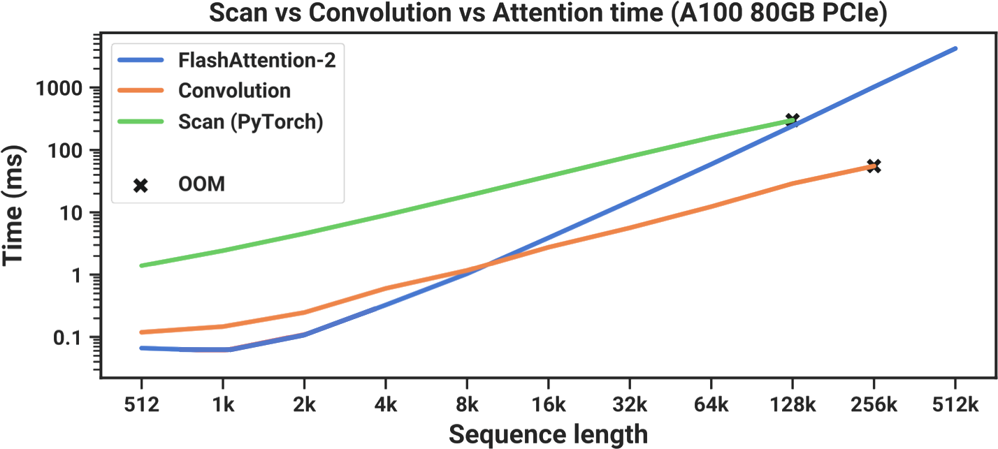
In the figure above, you can see that their PyTorch-based scan implementation (green) is always slower than FlashAttention-2 (blue), the fastest available “exact Attention” implementation.6 At a sequence length of 128,000 tokens, where the scan almost seems to catch up in runtime, it runs out of memory. In order for Mamba to be practical, it needed to be faster. This brought Mamba’s authors to Dao’s prior work on FlashAttention.
Review: FlashAttention
FlashAttention is a very fast implementation of Attention. When published, FlashAttention trained BERT-large 15% faster than the previous fastest training time, and it was 3 times faster than the widely-used HuggingFace implementation of GPT-2.
In a nutshell, FlashAttention’s key insight has to do with the speeds at which different operations run on your GPU. They realized that some GPU operations are compute-bound, meaning they are limited by the speed at which your GPU performs computations. However, other operations are memory-bound, meaning they are limited by the speed at which your GPU is able to transfer data.
Imagine you and a friend are playing a game: your friend has to run 50 meters to deliver two numbers to you, which you then need to multiply by hand. A timer starts when your friend begins running, and ends when you get the answer. Let’s say the numbers you need to multiply are 439,145,208 and 142,426,265. It would take you awhile to multiply these by hand. Your friend might take 5 seconds to deliver the numbers, but you might take 60 seconds to perform the multiplication. As a result, you are both compute-bound, since most of your time is spent on computation. Now, imagine the numbers you need to multiply are 4 and 3. While your friend still takes 5 seconds to run 50 meters, you can compute this result instantly. Now, you are both memory-bound, since most of your time is spent transferring data.
In this analogy, your GPU is essentially racing to move data into the right places to perform its computations. For example, let’s consider a masking operation. To compute a masked vector, your GPU simply needs to erase data values whenever the mask is equal to zero (and keep them the same whenever it is equal to one). If we used \(\boldsymbol{\oslash}\) to denote a masking operation, an example of this would be as follows, where the mask forces us to set the last three data elements to zero:
\[ \begin{pmatrix} 4 & 9 & 4 & 1 & 2 & 7 \end{pmatrix} \hspace{0.1cm}\boldsymbol{\oslash}\hspace{0.1cm} \begin{pmatrix} 1 & 1 & 1 & 0 & 0 & 0 \end{pmatrix}=\boxed{\begin{pmatrix} 4 & 9 & 4 & 0 & 0 & 0 \end{pmatrix}} \]
Since this is extremely easy to compute, your GPU ends up spending most of its time transferring memory, to move the data and mask matrices into the right places for computation. This means that masking is memory-bound. On the other hand, matrix multiplication involves lots and lots of additions and multiplications. Because so much more time is spent on computation than memory transfers, matrix multiplication is compute-bound. With this in mind, let’s look at a breakdown of the computations performed during Attention (matmul = matrix multiplication).
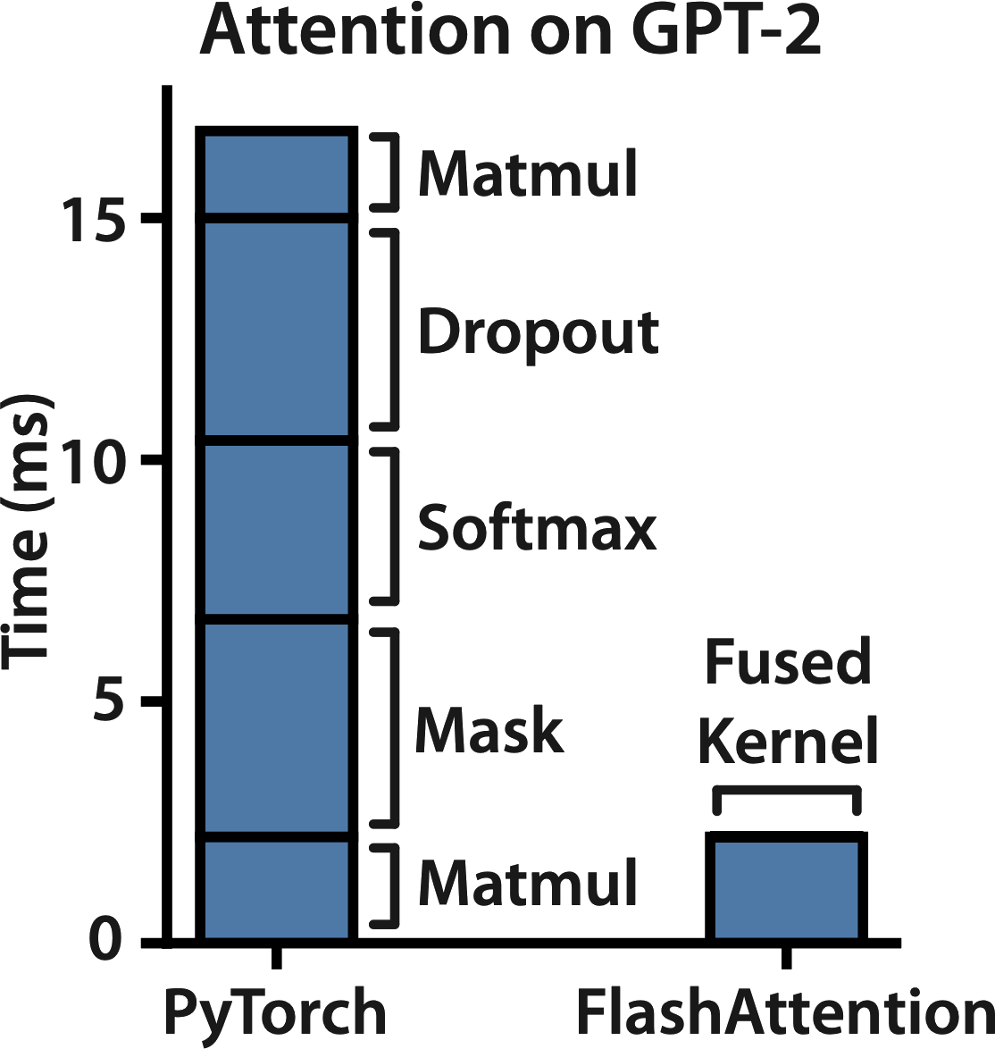
It turns out that dropout, softmax, and masking, which make up the bulk of Attention’s runtime, are all memory-bound. This means that most of the time we spend computing Attention is simply spent waiting for your GPU to move around data. With this in mind, I assume FlashAttention’s authors wondered, how can we speed up operations that are bounded by the speed of memory transfers?
This led FlashAttention’s authors to another key realization: GPU memory has two major regions. One of these, high-bandwidth memory (HBM), is really big, but really slow. The other one, static random-access memory (SRAM), is really small, but really fast. Let’s break down the differences between these regions on an A100 GPU:
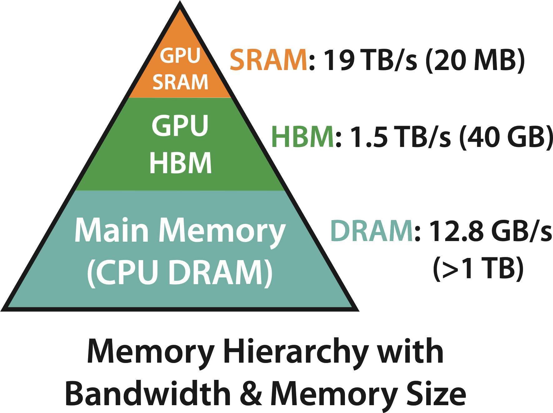
FlashAttention’s authors realized that you can compute memory-bound operations more efficiently if you’re extra careful about how you use these regions of GPU memory. They use an approach called tiling, in which small portions of your data are moved from HBM (slower) to SRAM (faster), computed in SRAM, and then moved back from SRAM to HBM. This makes FlashAttention really, really fast, while still being numerically equivalent to Attention.
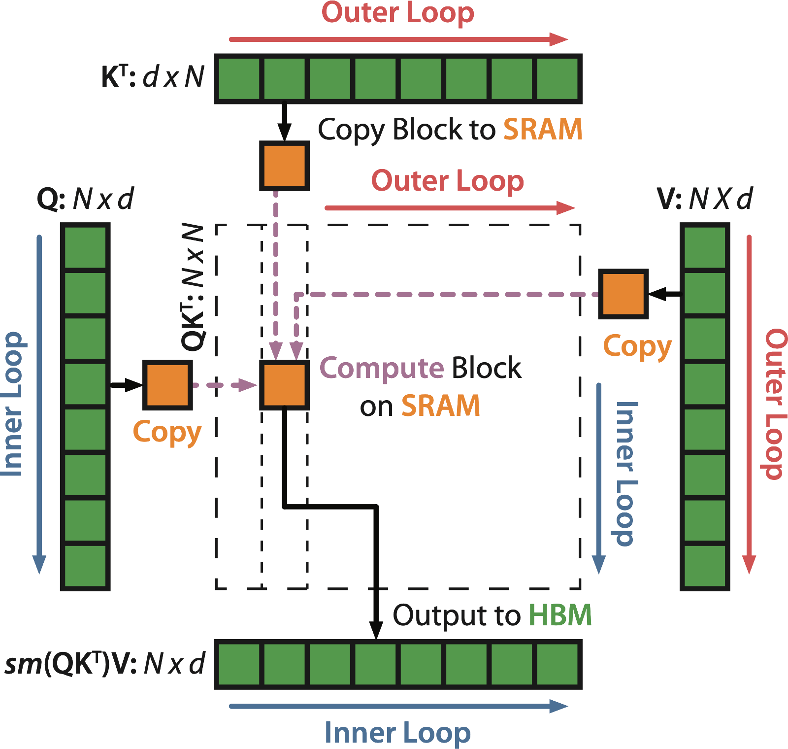
The details of how this works are fascinating, and I encourage you to check out the FlashAttention paper to learn more. However, for the purpose of understanding Mamba, this is basically all you need to know.
Back to Mamba
Remember that before we started this tangent on FlashAttention, we were trying to speed up our parallel scan implementation. Here is the same graph from earlier, where we can see that the scan implementation in PyTorch (green) is always slower than FlashAttention, the fastest “exact” Transformer (blue).7
It turns out that if you take this same memory-aware tiling approach when computing a scan, you can speed things up a lot. With this optimization in place, Mamba (red) is now faster than FlashAttention-2 (blue) at all sequence lengths.
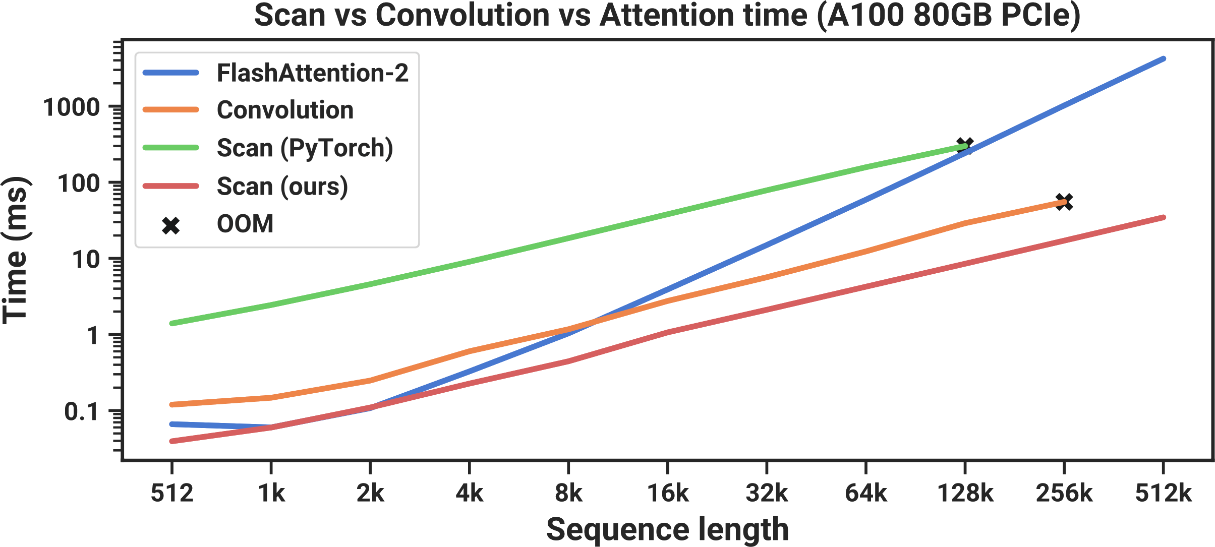
These results show that as far as speed goes, Mamba is practical, operating at a faster speed than the fastest exact Transformers. But is it any good at language modeling?
Results
Gu and Dao evaluate Mamba on a number of sequence modeling tasks involving language, genomics, and audio. I’m not as familiar with the latter two domains, but the results look cool: Mamba establishes state-of-the-art performance when modeling DNA from the Human Genome project, and audio from a piano music dataset. However, it’s the language results that have gotten many people excited. A lot of the online discourse about Mamba has focused on Figure 4, which I’ve included below.
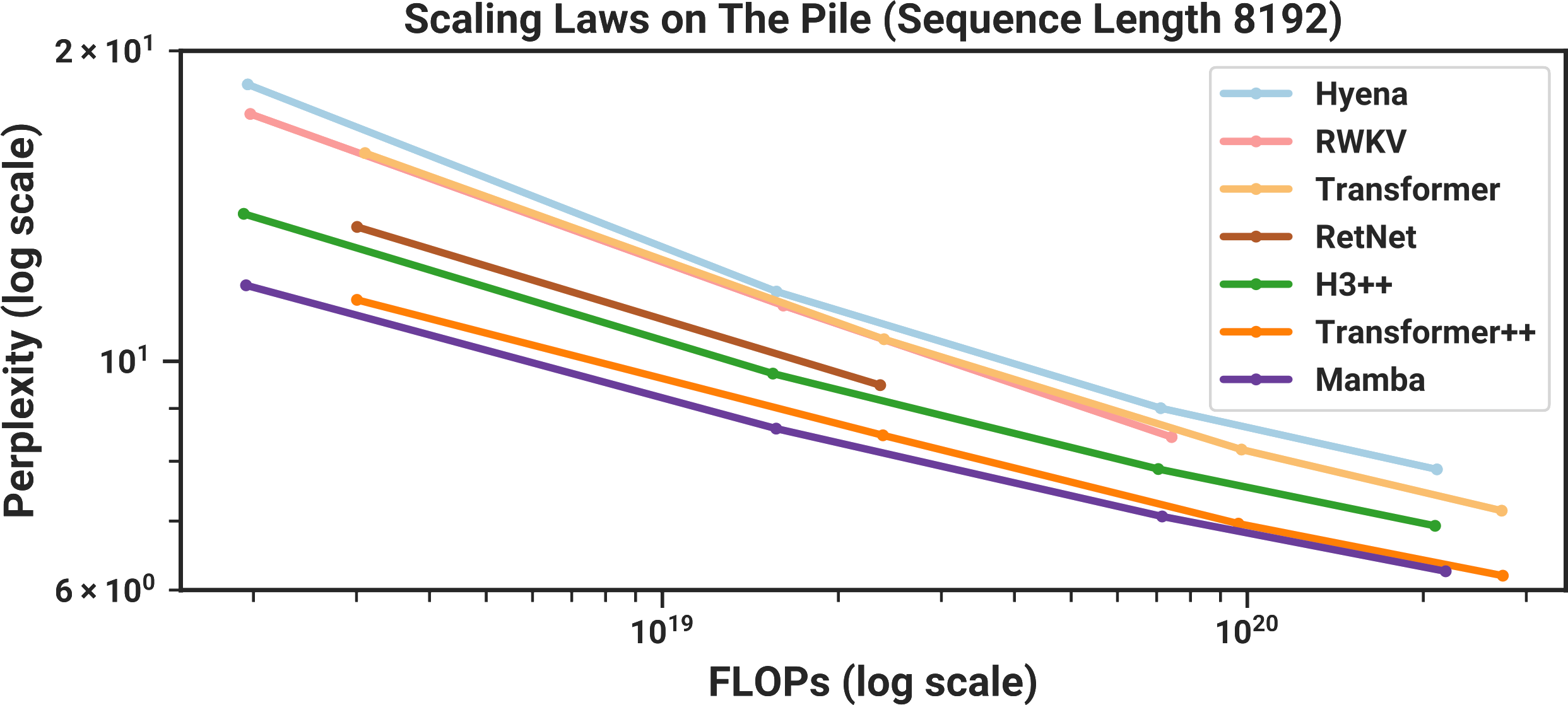
In this graph, model size increases to the right, and language modeling performance improves as you go further down.8 This means that the best models should be down and to the left: small (and therefore fast), and also very good at modeling language. Since Gu and Dao are academics, they don’t have thousands of GPUs available to train a GPT-4-sized model, so they made this comparison by training a bunch of smaller models, around 125M to 1.3B parameters. As the graph above shows, the results look really promising. When compared to other models of similar sizes, Mamba appears to be the best at modeling language.
What next?
I really enjoyed writing this blogpost, as I think Mamba innovates on language modeling in a pretty unique and interesting way! Unfortunately, a few reviewers didn’t agree: Gu and Dao planned to present Mamba at ICLR in May, but their paper was rejected a couple weeks ago, causing some bewildered reactions online.
Mamba apparently was rejected !? (https://t.co/bjtmZimFsS)
— Sasha Rush (@srush_nlp) January 25, 2024
Honestly I don't even understand. If this gets rejected, what chance do us 🤡 s have.
I would guess Gu and Dao are working now on the next version of the paper, and I would also imagine some companies with more GPUs than they know what to do with are currently trying to figure out whether Mamba’s performance holds up at larger model sizes. As we continue to want models that can process more and more tokens at once, linear-time models such as Mamba might someday provide an answer if they can demonstrate good performance. Until then, we can keep hacking away on our lame, old-school Transformers.